


Introduction to Motion Planning
-
Introduction to Motion Planning
- Prerequisites
- General Motivation
- What Navigation Means
- Local Versus Global Navigation
- The Basic Components of a Path Planning System
- Three possible Ways of Representing the Problem
- Searching the Graph
- Approach 1 — Road Maps
- Approach 2 — Cell Decomposition
- Approach 3 — An example without Graph: Potential Fields
- Comparing the Approaches
- Where This Leads
- Exercises
- Credits
- References
Prerequisites
- Graph definitions, representations, traversal and search — Section 0.2. Everything this section says about graphs, adjacency representations, BFS/DFS, Dijkstra and A* is defined and analysed there; here we only use those tools and show what they mean for a robot.
- Robot kinematics and configuration space — necessary to understand complexity of motion planning for robotic manipulators.
- Basic notions of low-level close-loop motion control, enough to understand how once one has planned a motion path, one can ensure that the robot tracks the path.
Definition. A robot is holonomic if it can move instantaneously in any direction of its configuration space: it can change each of its degrees of freedom independently, and the number of degrees of freedom it can control equals the number it has. An omnidirectional platform that can slide sideways is an example.
A robot is non-holonomic if some instantaneous motions are impossible even though every pose can eventually be reached. A car or a differential-drive robot cannot slide sideways, so it has to manoeuvre, for example by parallel parking, to get there.
General Motivation
You already use a motion planner several times a week. When you ask your phone how to get from the campus to the train station, it does not reason about asphalt, pedestrians or traffic lights: it reduces the city to a set of intersections and the road segments that connect them, attaches a number to each segment — travel time, distance, energy — and looks for the cheapest chain of segments between where you are and where you want to be. The answer it gives you is a plan; turning that plan into steering-wheel angles is somebody else’s job, and in the car that somebody is you.
A mobile robot faces exactly the same problem, minus the driver. A warehouse robot that must fetch a shelf sees a floor plan in which some squares are free and some are occupied; adjacent free squares are connected by feasible moves; some zones are slower than others and get a higher weight. Motion planning applies to all robots, whether on wheels, legs, or flying. A vacuum cleaner, a drone transporting blood samples from one place to another, and a robot arm reaching into a cluttered box are all, at bottom, asking the same question:
Given what I know about the world, what sequence of motions takes me from where I am to where I want to be without hitting anything?
What makes this a robotics problem rather than a graph-theory exercise is that the graph does not exist in advance. The world is continuous; the robot has a shape, a size and kinematic constraints; the map is incomplete and partly wrong. The real design decision is how to turn a continuous, cluttered, physical space into a discrete structure that an algorithm can search — and different answers to that question give the different families of planners presented in this chapter.
This section is the entry point to the chapter. It presents the classical, low-dimensional way of approaching the problem: build a graph that captures the connectivity of the free space, then search it. It is deliberately concrete — 2D maps, polygonal obstacles, grids you can draw on paper — because it makes the vocabulary (completeness, optimality, road map, cell decomposition, cost) tangible. The methods presented here are still the ones running inside most cleaning robots and warehouse fleets. They also run out of steam in a very specific and instructive way, which is precisely what motivates Sampling-Based Planning (Section 3.2) and the continuous, reactive formulations of Dynamical-Systems-Based Planning (Section 3.3).
What Navigation Means
Definition. Navigation is the problem of finding a collision-free path from one pose to another.
A pose is a position together with an orientation; a path is a continuous sequence of poses; the path is collision-free if no pose along it makes the robot intersect an obstacle.
Whenever you meet a navigation algorithm, three properties tell you most of what you need to know about it:
- Optimality — does the planner return trajectories that are optimal in some sense (length, execution time, energy consumption)? Optimal with respect to what is part of the question: the shortest path and the safest path are rarely the same path.
- Completeness — does the planner always find a solution when one exists (and report failure when none exists)? A complete planner never misses a feasible path; an incomplete one may.
- Offline / online — can the solution be computed in real time while the robot moves, or is it too heavy computationally and must be prepared in advance?
And three questions about the problem itself:
- Do we have a model of the environment (a map), or only the direction of the goal, for instance?
- If a map exists, are all the obstacles in it? (In practice: never.)
- Do we need to take into account the geometry, the kinematic constraints, and/or the dynamics of the robot?
An assumption you inherit. Most of the classical techniques presented in this section assume a mass-less, holonomic, point-like robot: no inertia, able to move in any direction instantly, and occupying no space at all. This is what makes them simple enough to teach on a slide — and it is also why a real implementation needs at least two extra ingredients even for simple real-world scenarios: a priori expansion of the obstacles by the radius of the robot (so that a path planned for a point is safe for a body), and low-level motion control to convert a geometric path into wheel commands. Keep this assumption in mind: half of the practical difficulties in this chapter come from relaxing it.
Local Versus Global Navigation
Navigation is traditionally split into two layers that answer different questions on different time scales.
| Local: obstacle avoidance | Global: path planning (motion planning) | |
|---|---|---|
| Role | Tactical: modulating the trajectory to avoid unforeseen, local obstacles | Strategic: planning the global trajectory |
| Knowledge | No map, or only a local, sensor-based one | A map (metric, grid-based or topological) and a goal location |
| Style | Rather reactive: no complex processing ⇒ fast | Rather cognitive: planning a series of actions ⇒ time consuming |
| Horizon | The next few centimetres or seconds | The whole mission |
Both are necessary in robotics, because environments are not fully predictable: sensors and maps are uncertain, and dynamic obstacles (people, other robots, a chair that moved) simply are not in the map. The global planner produces the intention; the local layer keeps the robot alive while it executes that intention.
This is the classic hybrid deliberative/reactive architecture: deliberative planning decomposes the task into sub-tasks, while behaviours execute reactively as a succession of sense–act couplings. Sensor data is routed both to the behaviours that need it and to the planner, which uses it to maintain a task-oriented world model.
Compared with industrial robotics in confined environments, mobile path planning is less complicated (far fewer degrees of freedom) but more frequent: the map and the real environment keep disagreeing, so the plan has to be recomputed again and again.
The Basic Components of a Path Planning System
To get a first grip on the problem, picture the simplest possible version of a mobile robot navigation system: a map handed to the robot in advance, a single plan computed once before departure, and a robot with no size and no dynamics. It is a deliberately naive picture — every section that follows, in this chapter and beyond, replaces one piece of it with something more capable — but it isolates the handful of building blocks that allow to create a primitive planning system:
- A global map of the environment, to know which positions are accessible and which are not.
- A start and an end position, expressed in that map.
- A path planning algorithm, to find a path within the map.
- A path following module, to track that path from start to goal. This requires knowing the position of the robot, in order to correct its motion — the controller determines the quality of the path following.
- A local navigation module, for reactive avoidance of everything the map does not contain.
When you drive to the station, your phone supplies 1–3, and you implement 4 and 5 as driver. An autonomous robot has to supply all five itself.
Keep this skeleton as a checklist for the rest of the chapter. The classical methods below — road maps, cell decompositions, potential fields — are all answers to block 3 alone, under the naive assumptions just stated. Relaxing those assumptions is exactly what the later sections do: Sampling-Based Planning (Section 3.2) scales block 3 to robots with many degrees of freedom; Dynamical-Systems-Based Planning (Section 3.3) folds blocks 3 and 4 into a single continuous process instead of plan-then-follow; and SLAM (Section 3.4) removes the assumption that block 1, the map, is given at all.
Three possible Ways of Representing the Problem
Everything that follows is a variation on one simple idea used to illustrate the components of the system: capture the connectivity of the free space into a graph, then search that graph for a path. The interesting part is how the graph is built.
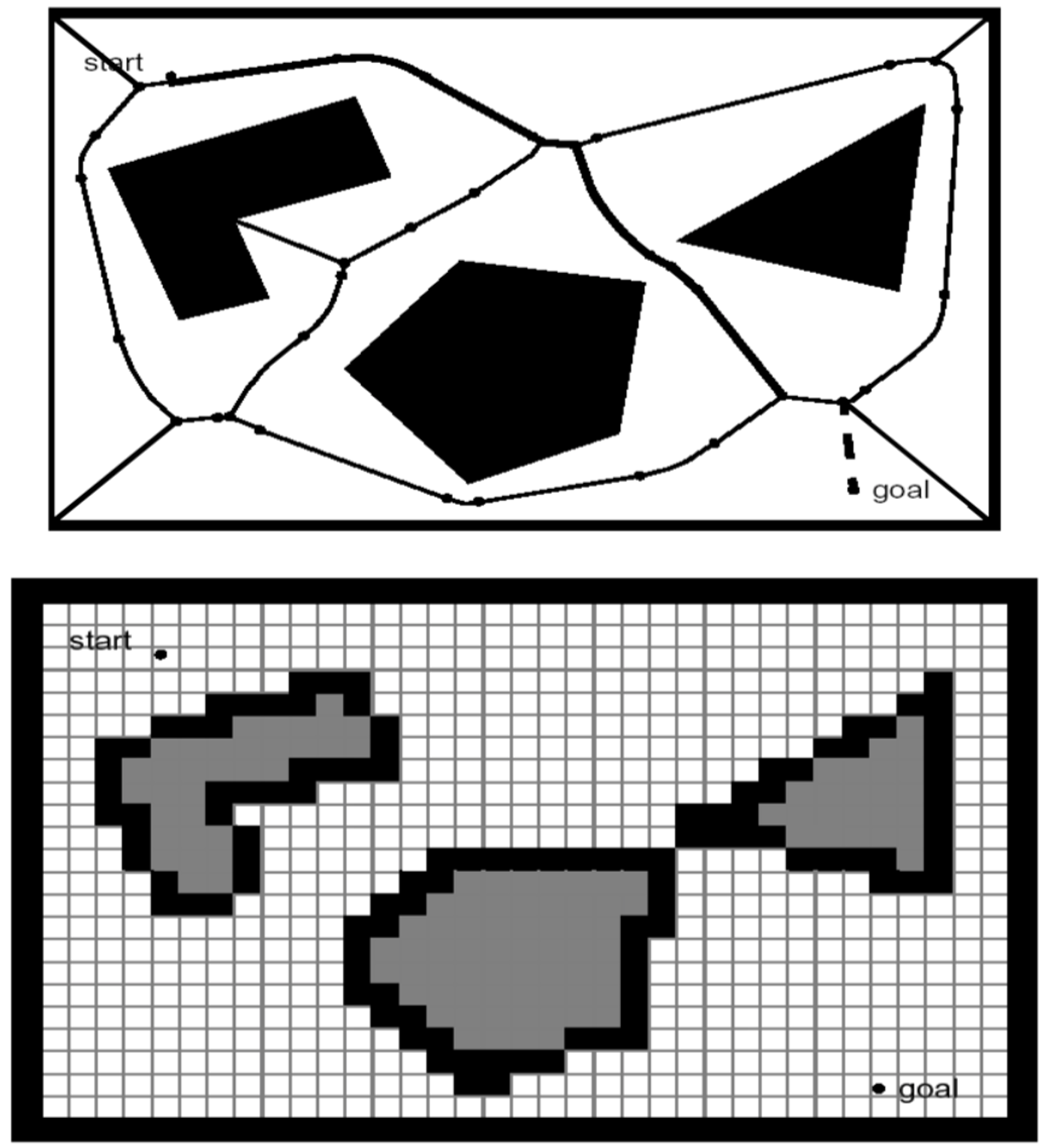
- Approach 1 — Road map. Identify a set of routes inside the free space (visibility graphs, Voronoi diagrams). Vertices are places worth passing through; edges are the routes between them.
- Approach 2 — Cell decomposition. Cut the space into cells, label each cell free or occupied, and connect adjacent free cells into a connectivity graph (exact decomposition, quadtrees, occupancy grids).
- Approach 3 — No graph at all. Define a continuous field over the space whose gradient points towards the goal (potential fields), and let the robot follow it.
In the first two cases the planning problem becomes a graph search problem, and it is exactly the graph search problem defined in Section 0.2: a weighted graph $G = (V, E)$, a source, a target, and a cost to minimise. This is worth stating plainly, because it is the single most useful idea in the chapter:
Whatever representation you choose, you transpose it into a graph and then you search the graph. Changing the representation changes the vertices, the edges and the weights — not the search.
Searching the Graph
Once the problem is a graph, it is searched with the standard algorithms — breadth-first, depth-first, Dijkstra, A* — and their definitions, correctness and complexity all belong to Section 0.2. What is specific to robotics is not the algorithms themselves but two implementation choices built on top of them: how the costs are designed, and how the search is adapted to the vehicle.
Cost design. On a grid, giving every cell the same cost turns Dijkstra into a simple wavefront expansion: a ripple that spreads outward from the start, one step at a time, until it reaches the goal, and the shortest path is then read off by walking downhill from the goal to the start. Real floors are rarely uniform, though — sand, water, gravel, a crowded corridor all cost more to cross than open pavement. Raising the cost of the difficult cells is enough; the search itself does not change, only the numbers written on the cells do.
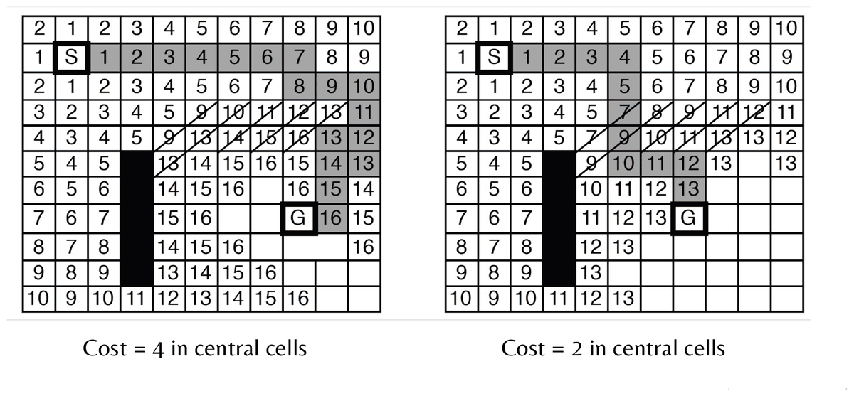
The robot’s behaviour was not programmed; it emerged from the weights. Choosing the cost function is therefore a modelling decision as important as choosing the algorithm: put a high cost near walls and the robot hugs the middle of corridors; put a high cost on turning and it prefers straight lines.
Adapting the search to the vehicle. A* is the search of choice for route finding, typically guided by the straight-line distance to the goal. Nothing forces the cells of its graph to be squares on a floor, or the moves to be “step north”: constraints on which cells are reachable, and on the transitions between them, can be added freely — a cost for turning, a maximum turning angle matching what the vehicle can actually do, a distinction between forward and backward motion. The resulting variant, Hybrid A*, is the standard way autonomous cars plan parking manoeuvres: the search algorithm has not changed, but the graph has, and with it the class of paths that can come out of it.
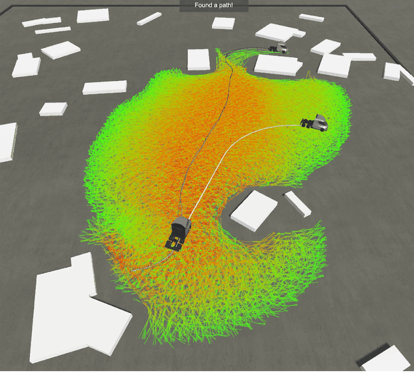
Image source: blog.habrador.com
Approach 1 — Road Maps
A road map keeps the space continuous and draws a small number of useful routes through it. The question is which routes deserve to exist.
Visibility Graphs
The challenge is to construct a set of roads that lets the robot go from start to goal while keeping the total number of roads small. The visibility graph answers it with a single rule: join every pair of vertices that can see each other — all obstacle corners, plus the start and the goal — by a straight segment that does not cross an obstacle.
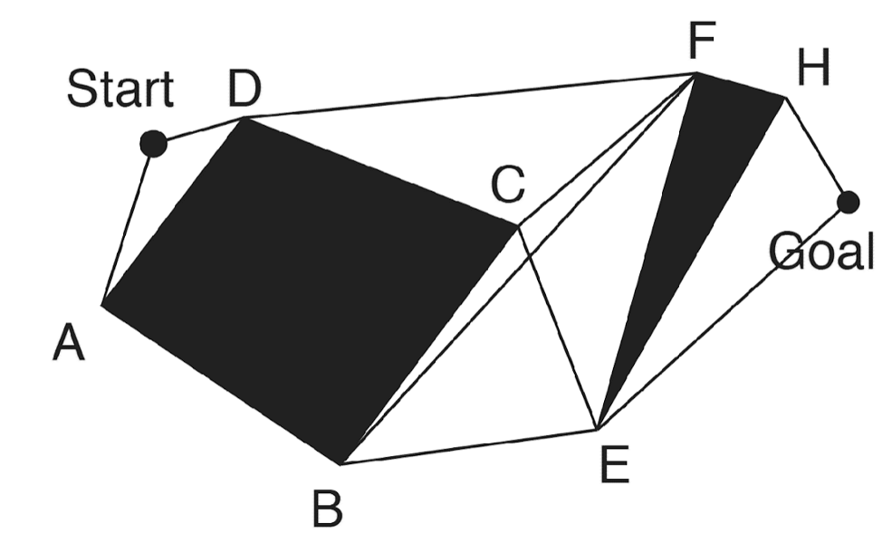
Why vertices, and only vertices? Because in a polygonal world the shortest way around an obstacle must touch it at a corner: any path that clears an obstacle by a margin can be shortened by pulling it tight against the corner. The corners are therefore the only places where an optimal path can bend, and a graph built on them loses nothing.
The construction turns the map into an ordinary graph — start, goal and corners become vertices; visible segments become edges:
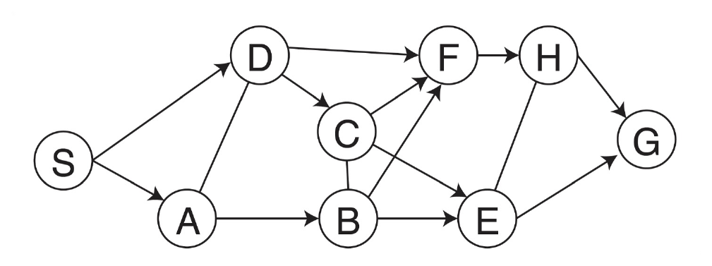
The edges now carry meaningful, unequal weights: the real Euclidean length of each segment. The distance from $S$ to $D$ is not the distance from $D$ to $C$.
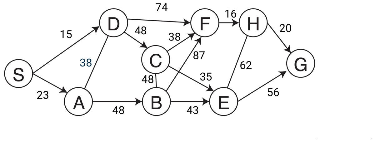
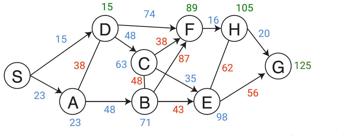
Finding the shortest path is then a matter of running Dijkstra (Section 0.2) on this weighted graph, from $S$ to $G$.
Properties.
- ✅ Complete — if a path exists, the visibility graph contains one.
- ✅ Optimal in path length — in a polygonal world it contains the shortest path, which is the strongest guarantee in this whole section.
- ❌ It grazes the obstacles. The optimal path runs along the corners, which for a robot with a body means scraping them.
The fix is the one announced earlier: grow the obstacles by the radius of the robot before building the graph, so that a path planned for a point is feasible for the real machine.
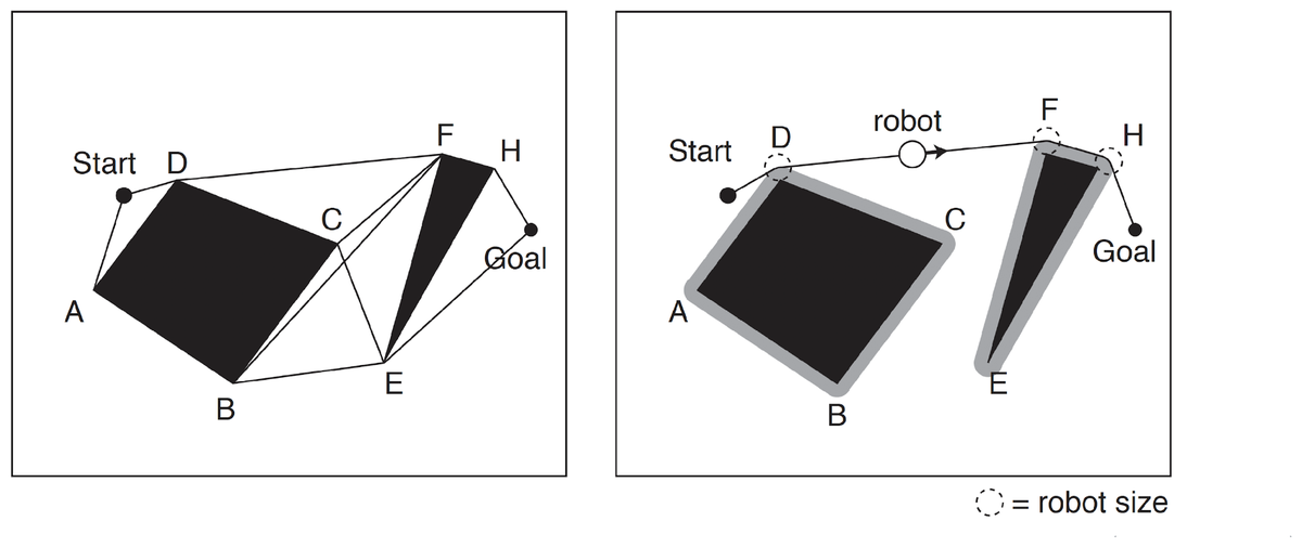
This “grow the obstacles, plan for a point” trick is the informal version of the configuration space construction, which is developed properly in Sampling-Based Planning. Everything in this section is happening in a two-dimensional configuration space without ever saying so.
Voronoi Diagrams
Visibility graphs take the shortest route and pay for it by hugging obstacles. The Voronoi diagram takes the opposite stance: stay as far away from everything as possible.
For each point of the free space, compute its distance to the nearest obstacle — think of circles growing out of every obstacle — and keep the points where two such circles meet. These are the points equidistant from two or more obstacles, and they form sharp ridges through the free space. When the obstacles are polygons, the Voronoi diagram consists of straight and parabolic segments.
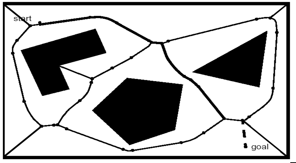
Properties.
- ✅ Tends to maximise the clearance between robot and obstacles.
- ✅ May be straightforward to execute with a range scanner: the robot simply maximises the local minima of its distance readings, which means it can follow the diagram without having computed it.
- ❌ Far from optimal in total path length — the robot systematically travels through the middle of the room where a straight line would do.
- ❌ May be problematic for localisation with short-range sensors, precisely because no obstacle may be sensed most of the time.
Approach 2 — Cell Decomposition
Instead of drawing roads, cut the free space into pieces. The recipe is always the same:
- Divide the free space into simple, connected regions called cells.
- Determine which open cells are adjacent, and build the connectivity graph — an ordinary graph in the sense of Section 0.2, whose vertices are cells rather than places.
- Find the cells containing the start and the goal, and search the connectivity graph for a path between them.
- From the sequence of cells, compute a trajectory inside each cell — for instance by passing through the midpoints of the cell boundaries, or by a sequence of line-following movements.
Two families exist: exact decompositions, where every cell is either completely free or completely occupied, and approximate ones, which do not take the geometry of the obstacles into account.
Exact Cell Decomposition
The boundaries between cells are placed at points of geometric criticality — typically the vertices of the obstacles, from which a vertical line is swept across the map. The underlying assumption is that the particular position of the robot inside a cell of free space does not matter.
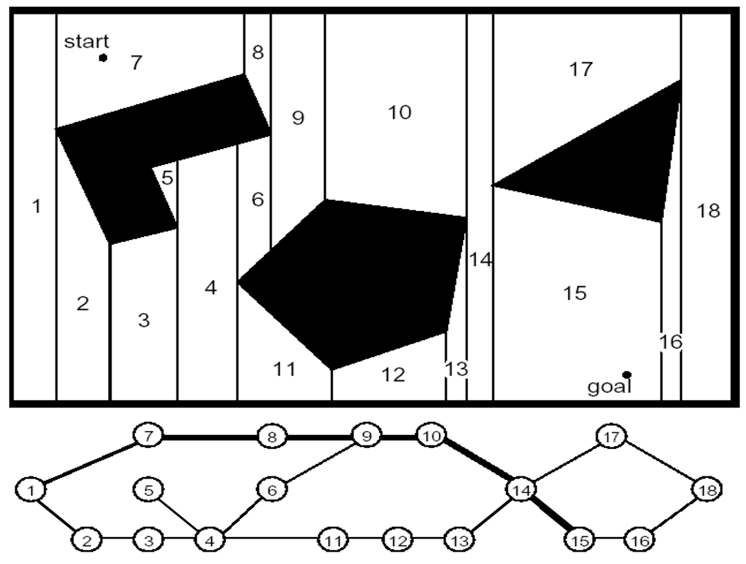
- ✅ The number of cells depends on the density and complexity of the objects, not on the size of the environment — an empty hall costs almost nothing.
- ✅ Complete.
- ❌ For the same reason, it is dependent on that density and complexity: a cluttered, non-polygonal environment becomes expensive and awkward.
- ❌ Crossing at boundary midpoints keeps the robot in the middle of free space, so — like Voronoi — the resulting path is not the shortest one.
Approximate: Adaptive Cell Decomposition
Forget the geometry and subdivide recursively instead. The rectangle covering the environment is cut into four identical rectangles. If the interior of a rectangle lies completely in free space or completely on an obstacle, it is not decomposed further; otherwise it is recursively cut into four again, and so on, stopping at a given minimal cell size. This is a quadtree.
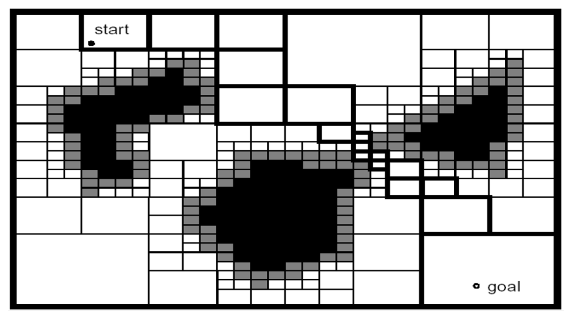
- ✅ Adapted to the complexity of the environment — resolution is spent where it is needed.
- ❌ May not be complete, depending on the minimal cell size: a passage narrower than the smallest cell is simply invisible.
- ❌ Navigation inside a large cell is no longer trivial, since cells have very different sizes.
Approximate: Fixed Grid-Size Decomposition
The simplest option of all, and by far the most used: cover the map with a regular grid, and mark a cell as occupied as soon as any obstacle intersects it. The result is an occupancy grid.
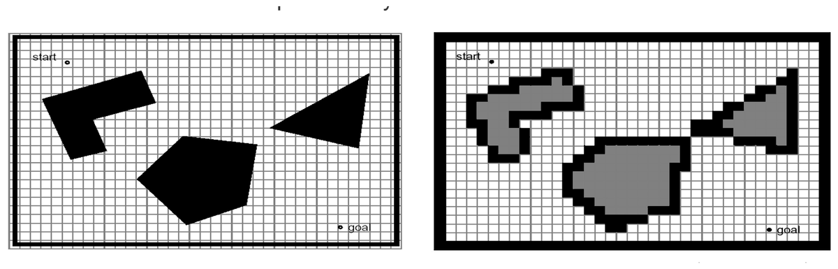
- ❌ Narrow passageways can be lost ⇒ may not be complete. A gap that the robot could physically fit through disappears if it is smaller than one cell.
- ✅ Extremely simple path planning algorithms — such as wavefront expansion, which is exactly constant-cost Dijkstra (Section 0.2) — can be applied directly ⇒ computationally efficient.
- ✅ Directly compatible with the way sensors build maps: turning a range reading into an update of the grid is simple — mark the cell it falls in as occupied, and the cells along the way as free — with no geometric fitting required, which is why the occupancy grid is the representation of choice in SLAM (Section 3.4).
Note that this brings us full circle: the grid we used to introduce Dijkstra was itself a cell decomposition. The grid is not “the map”, it is one representation choice among several, and its resolution is a trade-off between completeness and cost.
Approach 3 — An example without Graph: Potential Fields
A third possible approach abandons the graph entirely. The robot is treated as a particle under the influence of an artificial potential field: the goal generates an attractive force, and the obstacles generate repulsive forces. At every location, the direction obtained by the addition of all forces, is taken as the most promising direction of motion.
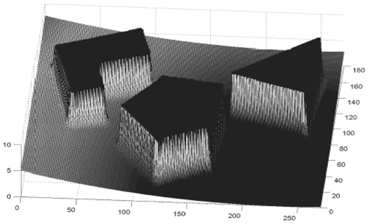
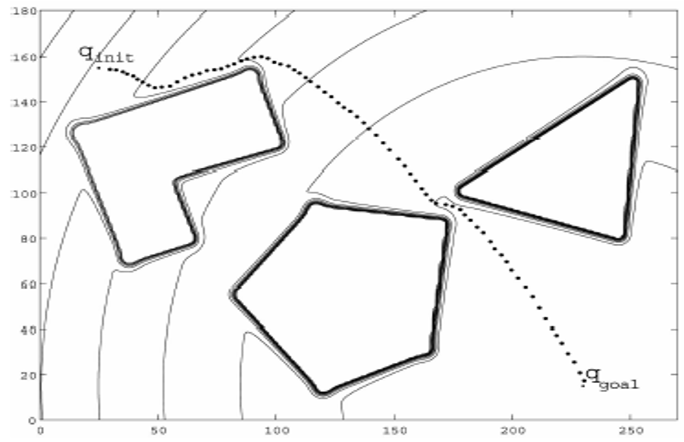
From force to wheels. If the robot is holonomic, the control is immediate: set the robot velocity $(v_x, v_y)$ proportional to the force $F(q)$, assuming the dynamics are negligible. If the robot is non-holonomic, a transformation is needed. For a differential-drive robot, for instance, the rotation speed can be set proportional to the angle $\alpha$ between $F(q)$ and the current orientation of the robot, while the forward speed is set proportional to $|F(q)|$ or to $|F(q)|\cos(\alpha)$ — the cosine term preventing the robot from driving fast in a direction it is not yet facing.
Interactive demo: EPFL Mobile Robots course, via calerga.ch
Notes on potential fields.
- ❌ Potential field methods are usually incomplete: a path may well exist that the method never finds.
- ❌ The local minimum problem is intrinsic — the sum of an attractive and several repulsive fields can create a basin that is not the goal, resulting in oscillations or dead-locks.
- ❌ The problem becomes more complex if the robot cannot be considered as a point mass.
- ✅ Easy to implement, efficient and reasonably reliable planners.
- ✅ Can be used offline to draw a complete path that is then followed by a low-level controller.
- ✅ Can be used online, computing only the force at the current pose and controlling the robot accordingly — the same code then serves as a local obstacle-avoidance layer.
Comparing the Approaches
| Method | Representation | Complete? | Optimal? | Needs a map? | Typical use |
|---|---|---|---|---|---|
| Visibility graph | Road map | ✅ Yes | ✅ Shortest path | Yes, polygonal | Known, structured, polygonal environments |
| Voronoi diagram | Road map | ✅ Yes | ❌ Maximises clearance instead | Yes | Safe navigation with range sensors |
| Exact cell decomposition | Cells | ✅ Yes | ❌ Mid-boundary paths | Yes, polygonal | Coverage, structured indoor maps |
| Adaptive (quadtree) | Cells | ⚠️ Up to the minimal cell size | ❌ Resolution-limited | Yes | Large maps with sparse obstacles |
| Fixed grid / occupancy | Cells | ⚠️ Up to the resolution | ❌ Resolution-limited | Yes | The workhorse; sensor-built maps, SLAM |
| Potential field | None (continuous field) | ❌ No (local minima) | ❌ No | No | Reactive control, online avoidance |
Where This Leads
Every method in this section shares two assumptions that are easy to miss because they are never stated: the world is two-dimensional, and the map is given. Lift either one and the picture changes.
- Lift the dimension. A grid is affordable in 2D and hopeless beyond it. Discretising each joint of a 7-degree-of-freedom arm into a mere 100 steps already yields $100^7 = 10^{14}$ cells — a graph no computer will build, let alone search. This is the curse of dimensionality, and it is what makes Sampling-Based Planning (Section 3.2) necessary: rather than enumerating the free space, sample it.
- Lift the discretisation. Potential fields showed that a continuous vector field can generate motion without any graph.
- Lift the map. All of the above assumed one. Building it while using it is SLAM (Section 3.4).
Exercises
Conceptual Exercise — Which family does it belong to?
Drag each method into the family it belongs to:
Exercise 1: Dijkstra with a Difficult Region
A robot moves on a $5 \times 7$ grid (rows $0..4$, columns $0..6$), 4-connected, starting at $(2,0)$ and ending at $(2,6)$. Entering a normal cell costs $1$. The cells with rows $1..3$ and columns $2..4$ are covered in sand, and entering one of them costs $s$.
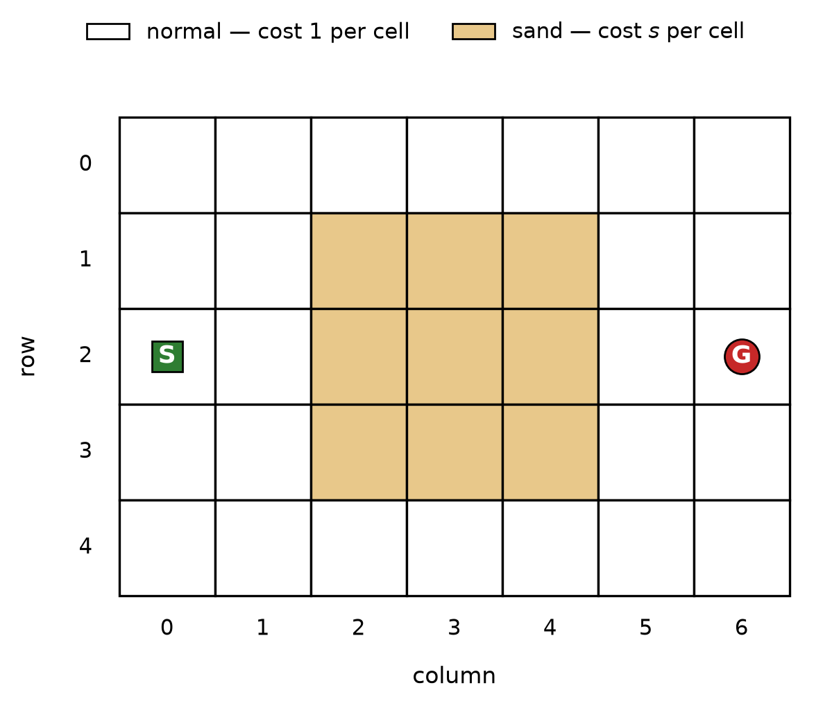
- What is the cost of the straight path through the sand, as a function of $s$?
- What is the cost of the cheapest path that avoids the sand entirely?
- For which values of $s$ does Dijkstra return the path through the sand?
- The optimal detour is not unique. Why, and does that matter?
Hints
- Count the cost of entering each cell; the start cell is free.
- The straight path enters exactly three sand cells.
- Rows $0$ and $4$ are entirely outside the sand.
Solution
-
Straight path: $(2,1)$ costs $1$, then three sand cells cost $s$ each, then $(2,5)$ and $(2,6)$ cost $1$ each: $$ C_{\text{through}} = 3s + 3 . $$
-
Going around by row $0$: two steps up, six steps across, two steps down, all at unit cost: $$ C_{\text{around}} = 2 + 6 + 2 = 10 . $$
-
The straight path wins when $3s + 3 < 10$, i.e. $s < 7/3 \approx 2.33$. With integer costs: $s \in {1, 2}$ goes through, $s \ge 3$ goes around. This is exactly the behaviour of Figure 2, where $s = 4$ sends the path around and $s = 2$ sends it through.
-
The detour by row $4$ has the same cost of $10$ by symmetry, and several interleavings of “up” and “right” moves also cost $10$. Dijkstra returns an optimal path, not the optimal path; ties are broken by the order in which cells happen to be expanded. It does not matter for the cost, but it does matter for reproducibility — and if you care about the shape of the path (fewer turns, more clearance), you must encode that preference in the cost function rather than hope for a good tie-break.
Exercise 2: The Size of a Visibility Graph
An environment contains polygonal obstacles with $V$ vertices in total, plus a start and a goal.
- How many vertices does the visibility graph have? How many candidate edges must be tested for visibility, in the worst case?
- Evaluate this for $V = 12$ and for $V = 200$.
- The robot is a disc of radius $r$. What must be done before building the graph, and what happens to a corridor whose width is smaller than $2r$?
- Why is it enough to consider only the obstacle vertices, and never a point in the middle of an obstacle edge?
Solution
-
The graph has $n = V + 2$ vertices. Every pair must be tested for mutual visibility, so the number of candidate edges is $$ \binom{n}{2} = \frac{(V+2)(V+1)}{2}, $$ and each test must be checked against all obstacle edges — which is why naive implementations are $\mathcal{O}(n^3)$ and why visibility graphs do not scale to cluttered scenes.
-
For $V = 12$: $\binom{14}{2} = 91$ candidate edges. For $V = 200$: $\binom{202}{2} = 20{,}301$. The quadratic growth is immediate.
-
The obstacles must be dilated by $r$ (a Minkowski sum with the robot disc) before the graph is built. A corridor narrower than $2r$ closes completely under this dilation, so the planner correctly reports that the robot cannot pass — the passage was never traversable in the first place.
-
In a polygonal environment, any collision-free path that clears an obstacle can be shortened by pulling it taut; a taut path is a polyline that bends only where it touches an obstacle, and it can only touch a convex corner. Points in the middle of an edge are therefore never needed for an optimal path.
Exercise 3: Resolution and Completeness
A robot of diameter $30\ \text{cm}$ navigates a building mapped as an occupancy grid. A cell is marked occupied as soon as any part of an obstacle falls inside it.
- With a cell size of $50\ \text{cm}$, what is the narrowest doorway the planner is guaranteed to recognise as passable?
- Give one scenario in which the planner reports “no path” although a path exists, and one in which it plans a path the robot cannot execute.
- The map is $100\ \text{m} \times 100\ \text{m}$. How many cells at $50\ \text{cm}$? At $5\ \text{cm}$? What does this suggest about “just use a finer grid”?
- Which of the three families of approaches would you use for a robot that must find the narrowest gaps in a static, well-surveyed, polygonal environment?
Solution
-
In the worst case the doorway is not aligned with the grid, so a free cell of $50\ \text{cm}$ can require up to $100\ \text{cm}$ of clear width to appear. Nothing narrower than that is guaranteed to be recognised, even though the robot only needs $30\ \text{cm}$.
-
False negative: a $40\ \text{cm}$ gap straddling a cell boundary marks both cells occupied, so the passage disappears and the planner declares failure although the robot would fit. False positive: a thin obstacle — a chair leg, a glass wall — that the sensor did not see leaves the cell marked free, and the planner routes the robot straight into it. The grid is only as good as what was written into it.
-
At $50\ \text{cm}$: $200 \times 200 = 4 \times 10^4$ cells. At $5\ \text{cm}$: $2000 \times 2000 = 4 \times 10^6$ cells, a hundred times more for one added decimal of precision. In 2D this is still affordable; the same refinement in the 7-dimensional configuration space of an arm multiplies the cost by $10^7$. Resolution is not free, and it is the first symptom of the curse of dimensionality.
-
A road-map approach, specifically a visibility graph on obstacles grown by the robot radius: it is exact, it is complete, it finds the shortest path, and — unlike any grid — it cannot lose a narrow gap, since a gap that survives the dilation is still connected in the graph.
Exercise 4: A Local Minimum You Can Draw
A point robot is at $q$, the goal is at $q_g$, and two circular obstacles of equal radius sit side by side, centred symmetrically on the segment $q q_g$, leaving a gap between them.
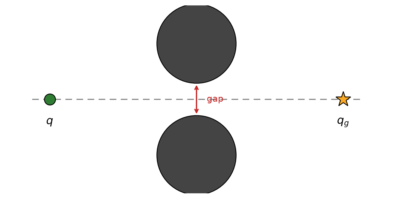
- Sketch the attractive force, the two repulsive forces, and their sum along the axis of symmetry.
- Show that a point exists on that axis where the total force vanishes, and explain why the robot stops there even though the gap is passable.
- Is this an artefact of the particular functions chosen, or something more fundamental?
- Name two practical remedies, and state the price of each.
Solution
-
On the axis of symmetry the two repulsive forces have equal magnitude and mirrored directions, so their lateral components cancel exactly and only a component pointing back along the axis survives. The attractive force points forward along the same axis.
-
The backward repulsive component grows without bound as the robot approaches the obstacles, while the attractive component is bounded (or grows only linearly). By continuity there is a point where they are equal and opposite: $F(q) = 0$. This is a local minimum of $U$, not the goal. The gradient carries no information about the gap, so the robot stops — or oscillates around the point if there is any noise.
-
Fundamental. Any smooth potential with several repulsive sources will generically have critical points other than the goal; a field guaranteed to have a single minimum is a navigation function, and constructing one requires global knowledge of the free space — which is exactly what the potential field method was trying to avoid.
-
(a) Add a random or rotational perturbation to escape the minimum: cheap, but it destroys any guarantee and can undo progress. (b) Use the potential field only as a local layer under a global planner that has a graph: robust, at the cost of needing a map and a planning step — which is the architecture described at the beginning of this section. A third route is to reshape the dynamics so that obstacles are circumvented rather than repelled.
Credits
This section is based on the lecture Mobile Robots 4/5 — Navigation given by Prof. Francesco Mondada, EPFL, in the Introduction to Robotics course, and on the recording of that lesson. It was prepared with the support of IEEE RAS and EPFL.
Several figures are adapted from the course slides, which themselves follow the presentation of Siegwart, Nourbakhsh & Scaramuzza, Introduction to Autonomous Mobile Robots (MIT Press).
References
- Siegwart, R., Nourbakhsh, I. R., & Scaramuzza, D. (2011). Introduction to Autonomous Mobile Robots (2nd ed.). MIT Press.
- Latombe, J.-C. (1991). Robot Motion Planning. Kluwer Academic Publishers.
- LaValle, S. M. (2006). Planning Algorithms. Cambridge University Press. Available at: https://lavalle.pl/planning/
- Choset, H., Lynch, K. M., Hutchinson, S., Kantor, G., Burgard, W., Kavraki, L. E., & Thrun, S. (2005). Principles of Robot Motion: Theory, Algorithms, and Implementations. MIT Press.
- Dijkstra, E. W. (1959). A note on two problems in connexion with graphs. Numerische Mathematik, 1, 269–271.
- Hart, P. E., Nilsson, N. J., & Raphael, B. (1968). A formal basis for the heuristic determination of minimum cost paths. IEEE Transactions on Systems Science and Cybernetics, 4(2), 100–107.
- Lozano-Pérez, T., & Wesley, M. A. (1979). An algorithm for planning collision-free paths among polyhedral obstacles. Communications of the ACM, 22(10), 560–570.
- Ó’Dúnlaing, C., & Yap, C. K. (1985). A “retraction” method for planning the motion of a disc. Journal of Algorithms, 6(1), 104–111.
- Khatib, O. (1986). Real-time obstacle avoidance for manipulators and mobile robots. The International Journal of Robotics Research, 5(1), 90–98.
- Dolgov, D., Thrun, S., Montemerlo, M., & Diebel, J. (2010). Path planning for autonomous vehicles in unknown semi-structured environments. The International Journal of Robotics Research, 29(5), 485–501.