🔝​

Screw Theory

• Screw Theory
  • Prerequisites
    • Quick quiz — prerequisites check
  • General Motivation
    • Quick quiz — motivation
  • Course Content
    • Notations
      • Reference frames and suffixes
      • Skew and screw operators
        • Quick quiz — notation and 6D objects
    • Rotation, Exponentials, and Product of Exponentials
      • Rotation as the solution of a differential equation
      • Simple intuition: one point moving on a circle
      • How the rotational differential equation appears
        • Quick quiz — rotational generator
      • The matrix exponential
        • Quick quiz — matrix exponential
      • From rotations to rigid motions
      • Spatial and body-fixed twists (two equivalent descriptions)
        • Quick quiz — twists in $SE(3)$
      • Product of exponentials
      • Constructing joint screws from axis geometry (revolute / prismatic)
        • Quick quiz — POE and joint screws
      • From joint rates to end-effector twist (Jacobian)
        • Quick quiz — Jacobian columns
      • Body Jacobian (often the cleaner choice for link-body analysis)
      • Pose error and the log map (why screws help in IK)
        • Quick quiz — body Jacobian and log map
      • Singularities as linear dependence of screws
        • Quick quiz — singularity interpretation
      • Why this matters for screw theory
    • Summary
    • Temporary
      • How to use
        • Quick quiz — interactive screw sketch
  • Credits
  • Resources

Prerequisites

• Linear algebra: vectors, matrices, rank, and linear dependence
• Rigid-body kinematics: angular velocity, linear velocity, and reference frames
• Basic statics and mechanics: forces, moments, torques, and power

Quick quiz — prerequisites check

Answer the following questions, multiple options may be correct.

General Motivation

Classical robot kinematics usually begins by attaching frames to links and joints, then multiplying the corresponding transformations. This works well for many introductory problems, but it can also make the geometry of motion feel secondary. In a spatial robot, the essential question is not only where each frame is placed, but what motion each joint permits between two neighboring bodies. Screw theory begins precisely from this motion-centered viewpoint.

The key observation is that rigid-body motion in space has a natural axis-based structure. A finite displacement can be interpreted through a screw: a rotation about an axis combined with a translation along that axis. At the velocity level, the same idea appears as an instantaneous screw axis. Thus, screw theory gives us one geometric language for both displacement and velocity. Rotation, translation, and helical motion are no longer treated as unrelated cases; they become different forms of the same underlying object.

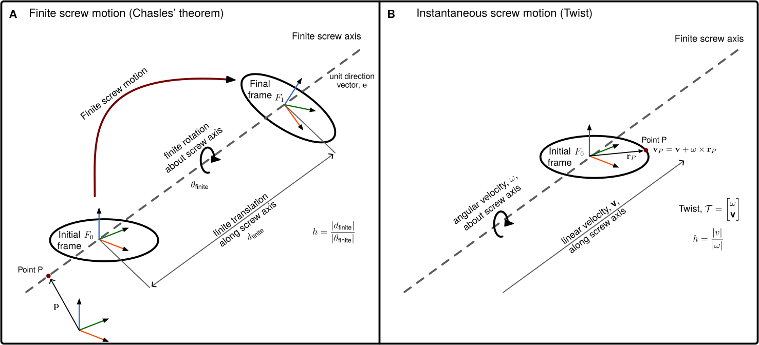
This viewpoint is especially useful in robotics because most elementary joints generate simple screw motions. A revolute joint corresponds to zero pitch, a prismatic joint corresponds to pure translation, and a helical joint corresponds to finite pitch. Therefore, instead of describing every joint through a special frame convention, we can describe it by its screw coordinates. For a joint axis with unit direction $\mathbf e$, a point $\mathbf p$ on the axis, and pitch $h$, the corresponding screw-coordinate vector $X$ is written as:

$$ X = \begin{bmatrix} \mathbf e \\
\mathbf p \times \mathbf e + h\mathbf e \end{bmatrix}. $$

The motion generated by this joint is then obtained through the exponential map which is the bridge from instantaneous motion to finite rigid-body motion. In other words, screw theory explains the geometry of the motion, while the exponential map provides the analytic mechanism that turns a joint coordinate into a rigid transformation.

The advantage becomes clearer for serial robots. A robot with $n$ revolute joints, ‘nR’ robot, is not merely a chain of ‘n’ frame transformations; it is a system generated by ‘n’ joint screws. Its reachable positions, velocity directions, and singular configurations are shaped by the geometry of these ‘n’ axes. For example, a 6R robot can be viewed as six screw generators acting in sequence.

Before composing these motions, we make the matrix form of a single joint motion explicit. Write the constant spatial joint screw as $Y_i=[\boldsymbol{\xi}_i^T\;\boldsymbol{\eta}_i^T]^T$, with angular part $\boldsymbol{\xi}_i$ and linear part $\boldsymbol{\eta}_i$, both represented in the fixed frame. Its hat denotes the following $4\times4$ matrix:

$$ \widehat{Y}_i= \begin{bmatrix} 0 & -\xi_{i,z} & \xi_{i,y} & \eta_{i,x} \\
\xi_{i,z} & 0 & -\xi_{i,x} & \eta_{i,y} \\
-\xi_{i,y} & \xi_{i,x} & 0 & \eta_{i,z} \\
0 & 0 & 0 & 0 \end{bmatrix}. $$

Let $\boldsymbol{\Omega}_i$ denote its upper-left $3\times3$ skew-symmetric block. The exponential is a $4\times4$ homogeneous transformation:

$$ \exp(\widehat{Y}_i\,q_i)= \begin{bmatrix} \mathbf{R}_i(q_i) & \mathbf{t}_i(q_i) \\
\mathbf{0}^T & 1 \end{bmatrix}. $$

For a revolute or helical joint, normalize the angular part so that $\lVert\boldsymbol{\xi}_i\rVert=1$; then $q_i$ is the rotation angle, and the blocks are

$$ \mathbf{R}_i(q_i)=\mathbf{I}_3 +\sin(q_i)\,\boldsymbol{\Omega}_i +(1-\cos(q_i))\,\boldsymbol{\Omega}_i^2, $$

$$ \mathbf{t}_i(q_i)= \left[q_i\mathbf{I}_3 +(1-\cos(q_i))\,\boldsymbol{\Omega}_i +(q_i-\sin(q_i))\,\boldsymbol{\Omega}_i^2\right]\boldsymbol{\eta}_i. $$

For a prismatic joint, $\boldsymbol{\xi}_i=\mathbf{0}$ and $\boldsymbol{\eta}_i$ is the unit translation direction. Here $q_i$ is a distance, and the matrix reduces to

$$ \exp(\widehat{Y}_i\,q_i)= \begin{bmatrix} \mathbf{I}_3 & q_i\boldsymbol{\eta}_i \\
\mathbf{0}^T & 1 \end{bmatrix}. $$

Thus each exponential contains a rotation block and a translation column. The end-effector motion is then written as a product of exponentials,

$$ \mathbf{H}_i(\mathbf q) = \exp(\widehat{Y}_1q_1)\exp(\widehat{Y}_2q_2)\cdots\exp(\widehat{Y}_iq_i)\mathbf{A}_i, $$

where $Y_j$ is the spatial screw-coordinate vector of joint $j$ represented in the inertial frame $\mathcal F_0$ at the reference configuration, and $\mathbf{A}_i=\mathbf{H}_i(\mathbf 0)$ is the absolute reference configuration of body $i$.

This formula is not only compact; it changes how we think about forward kinematics. The robot is described by its joint axes and reference pose, rather than by a long sequence of auxiliary frames. This reduces the dependence on restrictive conventions such as Denavit-Hartenberg parameters and makes the geometry of the mechanism more explicit.

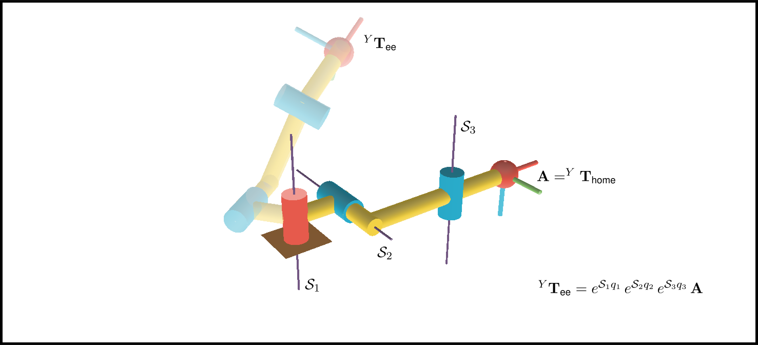
Screw theory also prepares the ground for velocity kinematics. The same screw coordinates that generate finite motions become the building blocks of twists and Jacobians. Each column of the geometric Jacobian can be interpreted as a joint screw transported to the current configuration. Singularities can then be studied as situations where the available joint screws lose rank or develop special geometric dependencies. This is why screw theory is more than a notation: it is a way to read the motion capability of a robot directly from the geometry of its axes.

For this chapter, the story is therefore simple. We start from the limitations of purely frame-based kinematics, introduce screws as the natural geometry of rigid-body motion, connect instantaneous and finite motion through the exponential map, and then use the Product of Exponentials formula to describe 3R and 6R robots. Once this language is established, twists, Jacobians, and singularities will appear as different views of the same geometric structure.

Exercise 5.1.2

Consider three one-degree-of-freedom joints: revolute, prismatic, and helical. For each joint, identify the screw axis direction $\mathbf e$, the pitch $h$, and the physical meaning of the exponential motion $\exp(\widehat{X}q)$. Then explain why a 6R robot can be interpreted as six screw-generated motions composed in sequence.

Quick quiz — motivation

Course Content

Notations

The following notations will be used throughout this chapter. They are fixed here so that the meaning of every symbol stays consistent as the ideas become more advanced.

• A scalar is written in standard italic form, for example $x \in \mathbb{R}$.
• A three-dimensional vector is written in bold lowercase, for example $\mathbf{r}, \mathbf{v}, \mathbf{f}$.
• A matrix is written in bold uppercase, for example $\mathbf{R}, \mathbf{J}, \mathbf{M}$.
• A vector quantity that is traditionally denoted by a Greek letter is written in bold Greek, for example the angular velocity $\boldsymbol{\omega}$.
• Six-dimensional screw-coordinate vectors use uppercase symbols such as $X$, $Y$, $V$, and $W$ and are written as stacked column vectors.
• The symbol $\phi$ denotes the scalar motion parameter. For a revolute motion it is an angle; later it can itself be a function of time, $\phi=\phi(t)$.
• A dot denotes a time derivative (e.g., $\dot{\phi}=d\phi/dt$), while $d(\cdot)/d\phi$ denotes differentiation with respect to the motion parameter.

Reference frames and suffixes

We use the same frame-index convention throughout:

• $\mathcal F_0$: the fixed (spatial/base) frame
• $\mathcal F_i$: a moving frame attached to body $i$

Whenever the coordinates of a vector, screw, twist, or wrench are represented in a particular frame, that frame is written as a left superscript:

• ${}^{0}\mathbf{a}$: coordinates of $\mathbf{a}$ represented in $\mathcal F_0$
• ${}^{i}\mathbf{a}$: coordinates of $\mathbf{a}$ represented in $\mathcal F_i$
• ${}^{0}V_i,\ {}^{i}V_i$: the same twist of body $i$ represented in $\mathcal F_0$ or $\mathcal F_i$
• ${}^{0}W,\ {}^{i}W$: a wrench represented in $\mathcal F_0$ or $\mathcal F_i$

The right subscript identifies the object, body, frame, or joint to which the quantity belongs. For a relative position vector we use the more specific convention

$$ {}^{k}_{i}\mathbf{r}_{j}, $$

which means: the vector from point $i$ to point $j$, represented in frame $\mathcal F_k$.

Homogeneous transformations and rotation matrices use the target-left/source-right convention:

• ${}^{i}\mathbf{R}_{j}\in SO(3)$ maps coordinates represented in $\mathcal F_j$ to coordinates represented in $\mathcal F_i$.
• ${}^{i}\mathbf{H}_{j}\in SE(3)$ is the pose of frame $\mathcal F_j$ relative to frame $\mathcal F_i$ and maps homogeneous coordinates from $\mathcal F_j$ to $\mathcal F_i$.

Concretely,

$$ {}^{i}\mathbf{a} = {}^{i}\mathbf{R}_{j}\,{}^{j}\mathbf{a}. $$

You can read ${}^{i}\mathbf{R}_{j}$ as “from $j$ to $i$”. Equivalently,

$$ {}^{j}\mathbf{R}_{i} = \left({}^{i}\mathbf{R}_{j}\right)^T = \left({}^{i}\mathbf{R}_{j}\right)^{-1}. $$

For absolute configurations, the fixed frame index is usually omitted:

$$ \mathbf{H}_i \equiv {}^{0}\mathbf{H}_i. $$

In a serial arm, frames $\mathcal F_0,\mathcal F_1,\dots,\mathcal F_n$ are attached to the ground and moving bodies. The same convention applies:

• ${}^{i}\mathbf{H}_{j}$ is the pose of frame $\mathcal F_j$ relative to frame $\mathcal F_i$.
• Composition: ${}^{i}\mathbf{H}_{k} = {}^{i}\mathbf{H}_{j}\,{}^{j}\mathbf{H}_{k}$.
• Inverse: ${}^{j}\mathbf{H}_{i} = ({}^{i}\mathbf{H}_{j})^{-1}$.

Skew and screw operators

We use two different “lift” operators:

• For a 3D vector $\mathbf{a}\in\mathbb{R}^3$, its skew-symmetric matrix is written with a tilde, $\widetilde{\mathbf{a}}\in\mathbb{R}^{3\times 3}$, defined by $\widetilde{\mathbf{a}}\,\mathbf{b}=\mathbf{a}\times \mathbf{b}$.
• For a six-dimensional screw/twist vector $X=\begin{bmatrix}\boldsymbol{\xi}\\ \boldsymbol{\eta}\end{bmatrix}$, its $4\times 4$ matrix in $\mathfrak{se}(3)$ is written with a hat, $\widehat{X}$.

In addition, we use the following symbols systematically:

• $X$: a generic screw-coordinate vector
• ${}^{i}X_i$: body-fixed joint screw coordinates of joint $i$, represented in $\mathcal F_i$
• $Y_i\equiv{}^{0}Y_i$: spatial joint screw coordinates of joint $i$, represented in $\mathcal F_0$
• $V$: a twist, that is, a motion screw
• $W$: a wrench, that is, a force screw
• $\boldsymbol{\xi}$: the upper three-dimensional component of a generic screw-coordinate vector
• $\boldsymbol{\eta}$: the lower three-dimensional component of a generic screw-coordinate vector
• $\mathbf{f}$: a force vector
• $\mathbf{m}$: a moment vector
• $\mathbf{v}$: a linear velocity vector
• $\boldsymbol{\omega}$: an angular velocity vector
• $\mathbf{e}$: a unit direction vector along a screw/rotation axis
• $\mathbf{p}$: a position vector to any point on a screw axis
• $h$: screw pitch
• ${}^{k}_{i}\mathbf{r}_{j}$: the position vector from point $i$ to point $j$, represented in $\mathcal F_k$
• $\mathrm{span}{X_1,\dots,X_k}$: the subspace generated by the listed screws

Accordingly, a generic screw is written as a stacked six-dimensional entity:

$$ X= \begin{bmatrix} \boldsymbol{\xi} \\
\boldsymbol{\eta} \end{bmatrix}. $$

For an axis with unit direction $\mathbf{e}$, a point $\mathbf{p}$ on the axis, and pitch $h$,

$$ X= \begin{bmatrix} \mathbf{e}\\
\mathbf{p}\times\mathbf{e}+h\mathbf{e} \end{bmatrix}. $$

When the screw represents motion, we write the twist as

$$ V= \begin{bmatrix} \boldsymbol{\omega} \\
\mathbf{v} \end{bmatrix}. $$

When it represents force transmission, we write the wrench as

$$ W= \begin{bmatrix} \mathbf{f} \\
\mathbf{m} \end{bmatrix}. $$

This stacked notation will be maintained throughout the chapter whenever a six-dimensional object is composed of two three-dimensional vectors.

To discuss reciprocity, we will use $\odot$ to denote the reciprocal product between two screws:

$$ X_1 \odot X_2 = \boldsymbol{\xi}_1 \cdot \boldsymbol{\eta}_2 + \boldsymbol{\xi}_2 \cdot \boldsymbol{\eta}_1. $$

In particular, for a wrench and a twist, the pairing becomes

$$ W \odot V = \mathbf{f}\cdot\mathbf{v} + \mathbf{m}\cdot\boldsymbol{\omega}. $$

This scalar is the quantity that will later encode power and reciprocity. A recurring idea in this chapter is that two screws are reciprocal when their pairing is zero.

Quick quiz — notation and 6D objects

Rotation, Exponentials, and Product of Exponentials

To make screw theory useful for robot kinematics, we need one more bridge: how an instantaneous motion gives rise to a finite motion. That bridge is provided by a differential equation and its solution through the matrix exponential.

Rotation as the solution of a differential equation

Before talking about screws in full generality, it helps to start with ordinary rotation.

The set $SO(3)$ is the set of all $3\times 3$ rotation matrices:

$$ SO(3) = { \mathbf{R} \in \mathbb{R}^{3 \times 3} \mid \mathbf{R}^T \mathbf{R} = \mathbf{I},\ \det(\mathbf{R}) = 1 }. $$

This notation means:

• $S$ stands for special, which here means determinant $+1$,
• $O$ stands for orthogonal, which means $\mathbf{R}^T\mathbf{R}=\mathbf{I}$,
• $(3)$ means we are in three-dimensional space.

So an element of $SO(3)$ is exactly a matrix that rotates vectors in 3D without stretching them, shrinking them, or reflecting them.

If a rigid body rotates, its orientation changes as the rotation angle accumulates, so we write

$$ \mathbf{R}(\phi)\in SO(3). $$

The main question is then:

If we know the body’s instantaneous angular velocity, how do we recover the finite rotation after some rotation angle?

That is where the differential equation appears.

Simple intuition: one point moving on a circle

First consider a point rotating in the $x$-$y$ plane around the origin with constant angular speed $\omega$, so the rotation angle is $\phi(t)=\omega t$. Parameterizing the position by the angle, we write

$$ \mathbf{r}(\phi) = \begin{bmatrix} \cos(\phi) \\
\sin(\phi)\\
0 \end{bmatrix} $$

From elementary kinematics, the velocity is tangent to the circle and perpendicular to the radius. In matrix form,

$$ \frac{d\mathbf{r}(\phi)}{d\phi}= \begin{bmatrix} 0 & -1 & 0 \\
1 & 0 & 0 \\
0 & 0 & 0 \end{bmatrix} \mathbf{r}(\phi) $$

«!– figure>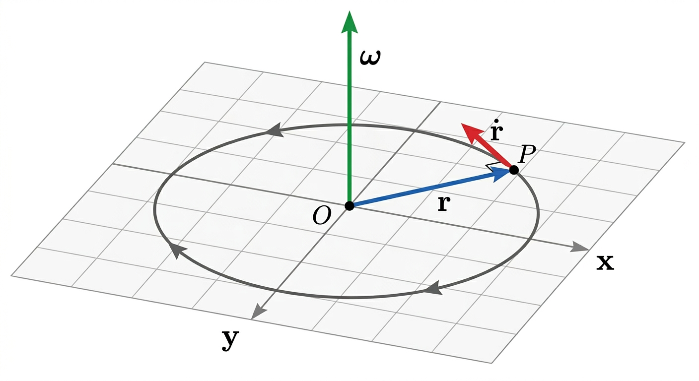

</figure> –>

So even in this simple planar case, the motion is already written as a linear differential equation of the form

$$ \frac{d\mathbf{r}}{d\phi} = \widetilde{\mathbf{e}}\,\mathbf{r}, $$

where $\mathbf{e}$ is the (unit) axis of rotation (here $\mathbf{e}=\mathbf{e}_3$) and $\widetilde{\mathbf{e}}$ is its skew-symmetric matrix.

The 3D case is the same idea, only now the generator is built from the angular velocity vector.

How the rotational differential equation appears

Using the skew-symmetric matrix associated with a unit rotation axis $\mathbf{e}$,

$$ \widetilde{\mathbf{e}} = \begin{bmatrix} 0 & -n_z & n_y \\
n_z & 0 & -n_x \\
-n_y & n_x & 0 \end{bmatrix}, $$

which is defined so that

$$ \widetilde{\mathbf{e}}\,\mathbf{a}=\mathbf{e}\times \mathbf{a} $$

for every vector $\mathbf{a}\in\mathbb{R}^3$.

Now take any vector $\mathbf{u}$ fixed in the body. As the body rotates, its coordinates in the spatial frame are

$$ \mathbf{r}(\phi)=\mathbf{R}(\phi)\mathbf{u}. $$

Its rate of change with respect to the rotation angle must be

$$ \frac{d\mathbf{r}(\phi)}{d\phi}=\mathbf{e}\times \mathbf{r}(\phi) = \widetilde{\mathbf{e}}\,\mathbf{r}(\phi). $$

But since $\mathbf{u}$ is constant in the body,

$$ \frac{d\mathbf{r}(\phi)}{d\phi}=\frac{d\mathbf{R}(\phi)}{d\phi}\mathbf{u}. $$

Combining the two expressions gives

$$ \frac{d\mathbf{R}(\phi)}{d\phi}\mathbf{u} = \widetilde{\mathbf{e}}\,\mathbf{R}(\phi)\mathbf{u} $$

for every body-fixed vector $\mathbf{u}$. Therefore,

$$ \frac{d\mathbf{R}(\phi)}{d\phi} = \widetilde{\mathbf{e}}\,\mathbf{R}(\phi). $$

This is the rotational differential equation with $\phi$ as the parameter. It says that the rate of change of orientation is produced by the infinitesimal rotation operator $\widetilde{\mathbf{e}}$ acting on the current orientation. (Later, if $\phi=\phi(t)$, then $\boldsymbol{\omega}=\dot{\phi}\,\mathbf{e}$ and the usual time-based form is recovered.)

If the axis is constant, this linear differential equation has the solution

$$ \mathbf{R}(\phi)=\exp(\widetilde{\mathbf{e}}\,\phi)\,\mathbf{R}(0). $$

This is the first important idea: a finite rotation is obtained by integrating an instantaneous rotational generator, and the result is written with the matrix exponential.

Quick quiz — rotational generator

The matrix exponential

For any square matrix $\mathbf{M}$, the exponential is defined by the power series

$$ \exp(\mathbf{M})= \mathbf{I}+\mathbf{M}+\frac{\mathbf{M}^2}{2!}+\frac{\mathbf{M}^3}{3!}+\frac{\mathbf{M}^4}{4!}+\cdots $$

So here we set

$$ \mathbf{M}=\widetilde{\mathbf{e}}\,\phi. $$

Then

$$ \exp(\widetilde{\mathbf{e}}\,\phi) = \mathbf{I} + \widetilde{\mathbf{e}}\,\phi + \frac{(\widetilde{\mathbf{e}}\,\phi)^2}{2!} + \frac{(\widetilde{\mathbf{e}}\,\phi)^3}{3!} + \frac{(\widetilde{\mathbf{e}}\,\phi)^4}{4!} +\cdots $$

Now use the identities for a unit vector $\mathbf{e}$:

$$ (\widetilde{\mathbf{e}})^2 = \mathbf{e}\mathbf{e}^T - \mathbf{I}, \quad (\widetilde{\mathbf{e}})^3 = -\widetilde{\mathbf{e}}, \quad (\widetilde{\mathbf{e}})^4 = -(\widetilde{\mathbf{e}})^2. $$

Hence the powers repeat in cycles:

$$ (\widetilde{\mathbf{e}})^{2k+1} = (-1)^k\widetilde{\mathbf{e}}, \quad (\widetilde{\mathbf{e}})^{2k+2} = (-1)^k(\widetilde{\mathbf{e}})^2. $$

Substituting into the power series gives

$$ \exp(\phi\widetilde{\mathbf{e}}) = \mathbf{I} + \left(\phi-\frac{\phi^3}{3!}+\frac{\phi^5}{5!}-\cdots\right)\widetilde{\mathbf{e}} + \left(\frac{\phi^2}{2!}-\frac{\phi^4}{4!}+\frac{\phi^6}{6!}-\cdots\right)(\widetilde{\mathbf{e}})^2. $$

Recognizing the sine and cosine series,

$$ \sin\phi = \phi-\frac{\phi^3}{3!}+\frac{\phi^5}{5!}-\cdots, \quad 1-\cos\phi = \frac{\phi^2}{2!}-\frac{\phi^4}{4!}+\frac{\phi^6}{6!}-\cdots $$

we obtain the Euler-Rodrigues formula:

$$ \exp(\phi\widetilde{\mathbf{e}}) = \mathbf{I} + \sin\phi\,\widetilde{\mathbf{e}} + (1-\cos\phi)\,(\widetilde{\mathbf{e}})^2. $$

So the exponential is not an abstract symbol only. It is the compact closed-form expression for the finite rotation generated by a rotation of angle $\phi$ about axis $\mathbf{e}$.

Placeholder image: angular velocity vector generating an infinitesimal rotation and the corresponding finite rotation.

Quick quiz — matrix exponential

From rotations to rigid motions

Rigid-body motion in space involves both orientation and position. We therefore move from the rotation group $SO(3)$ to the rigid-motion group $SE(3)$.

A rigid motion of body $i$ relative to the fixed frame $\mathcal F_0$ is written as the homogeneous transformation

$$ \mathbf{H}_i(\phi)\equiv{}^{0}\mathbf{H}_{i}(\phi)= \begin{bmatrix} {}^{0}\mathbf{R}_{i}(\phi) & {}^{0}_{0}\mathbf{r}_{i}(\phi) \\
\mathbf{0}^T & 1 \end{bmatrix} \in SE(3). $$

Here $\phi$ plays the role of a scalar motion parameter (for a revolute motion it is an angle; for a prismatic motion it is a distance).

Its motion per unit parameter $\phi$ is described by a twist. When represented in the fixed frame $\mathcal F_0$, we write

$$ {}^{0}V_i= \begin{bmatrix} {}^{0}\boldsymbol{\omega}_i \\
{}^{0}\mathbf{v}_i \end{bmatrix}, $$

To write this twist as a matrix, let ${}^{0}\boldsymbol{\omega}_i=[{}^{0}\omega_{i,x}\;{}^{0}\omega_{i,y}\;{}^{0}\omega_{i,z}]^T$. The tilde denotes the $3\times3$ skew-symmetric matrix

$$ \widetilde{\left({}^{0}\boldsymbol{\omega}_i\right)}= \begin{bmatrix} 0 & -{}^{0}\omega_{i,z} & {}^{0}\omega_{i,y} \\
{}^{0}\omega_{i,z} & 0 & -{}^{0}\omega_{i,x} \\
-{}^{0}\omega_{i,y} & {}^{0}\omega_{i,x} & 0 \end{bmatrix}. $$

Multiplying this matrix by a vector gives the cross product with ${}^{0}\boldsymbol{\omega}_i$. The equivalent $4\times4$ twist matrix is therefore

$$ {}^{0}\widehat{V}_i = \begin{bmatrix} \widetilde{\left({}^{0}\boldsymbol{\omega}_i\right)} & {}^{0}\mathbf{v}_i \\
\mathbf{0}^T & 0 \end{bmatrix}. $$

The rigid motion then satisfies the analogous differential equation

$$ \frac{d\mathbf{H}_i(\phi)}{d\phi} = {}^{0}\widehat{V}_i\,\mathbf{H}_i(\phi). $$

Spatial and body-fixed twists (two equivalent descriptions)

For kinematic analysis it is crucial to distinguish how a twist is represented.

Given a time-parameterized motion $\mathbf{H}_i(t)\equiv{}^{0}\mathbf{H}_{i}(t)$, we define:

• the spatial twist of body $i$, resolved in $\mathcal F_0$:

$$ {}^{0}\widehat{V}_i \;:=\; \dot{\mathbf{H}}_i\, \mathbf{H}_i^{-1}, $$

• the body-fixed twist of body $i$, resolved in $\mathcal F_i$:

$$ {}^{i}\widehat{V}_i \;:=\; \mathbf{H}_i^{-1}\, \dot{\mathbf{H}}_i. $$

They describe the same physical motion but in different coordinates. The two representations are related by the Adjoint mapping:

$$ {}^{0}V_i=\mathrm{Ad}_{\mathbf{H}_i}\,{}^{i}V_i, \qquad {}^{i}V_i=\mathrm{Ad}_{\mathbf{H}_i^{-1}}\,{}^{0}V_i. $$

If the twist is constant, the solution is

$$ \mathbf{H}_i(\phi)=\exp({}^{0}\widehat{V}_i\,\phi)\,\mathbf{H}_i(0). $$

This is the finite version of a twist. In other words, a constant twist generates a finite screw motion. Rotation appears as a special case; pure translation appears as another limiting case; and the general case combines both in one unified object.

Quick quiz — twists in $SE(3)$

Product of exponentials

Once a single joint motion is written as an exponential, a serial chain can be built by composing those exponentials one after another.

Constructing joint screws from axis geometry (revolute / prismatic)

To use the POE formula on an actual serial robot, we need the spatial joint screw coordinates $Y_i$ as a 6-vector $ Y_i= \begin{bmatrix}\mathbf{e}_i\\ \mathbf{y}_i\times\mathbf{e}_i+h_i\mathbf{e}_i\end{bmatrix}, $ where the coordinates are represented in the fixed frame $\mathcal F_0$.

In the chosen reference configuration (typically the home pose):

• Revolute joint about an axis with unit direction $\mathbf{e}_i$ passing through a point with position vector $\mathbf{y}_i$:

  $$ h_i=0, \qquad Y_i= \begin{bmatrix} \mathbf{e}_i\\
  \mathbf{y}_i\times\mathbf{e}_i \end{bmatrix}. $$

• Prismatic joint translating along unit direction $\mathbf{e}_i$:

  $$ Y_i= \begin{bmatrix} \mathbf{0}\\
  \mathbf{e}_i \end{bmatrix}. $$

These formulas are the practical bridge between “axis in space” drawings and the algebraic $\exp(\widehat{Y}_i q_i)$ factors used in POE.

Suppose joint $i$ is associated with the spatial screw $Y_i$ in the reference configuration. If its joint variable is $q_i$, then the motion contributed by that joint is written as

$$ \exp(\widehat{Y}_i\,q_i). $$

For a serial manipulator with $n$ joints, the end-effector configuration can therefore be written as

$$ \mathbf{H}_n(\mathbf{q}) = \exp(\widehat{Y}_1 q_1) \exp(\widehat{Y}_2 q_2) \cdots \exp(\widehat{Y}_n q_n)\, \mathbf{A}_n, $$

where $\mathbf{H}_n\equiv{}^{0}\mathbf{H}_n$ and $\mathbf{A}_n:=\mathbf{H}_n(\mathbf{0})$ is the absolute reference configuration of the end effector.

This expression is called the Product of Exponentials (POE) formula. Each factor represents one joint screw acting on the body, and the complete forward kinematics is obtained by multiplying these finite joint motions in sequence.

The conceptual advantage is important:

• the model is written directly in terms of geometric joint axes,
• revolute, prismatic, and helical joints are treated in one common language,
• the kinematics is expressed without needing restrictive coordinate conventions such as Denavit-Hartenberg tables.

Quick quiz — POE and joint screws

From joint rates to end-effector twist (Jacobian)

The POE formula gives finite pose as a function of joint variables. The Jacobian appears when we ask the corresponding instantaneous question:

Given joint velocities $\dot{\mathbf{q}}=\begin{bmatrix}\dot{q}_1 & \cdots & \dot{q}_n\end{bmatrix}^T$, what is the end-effector twist?

Step 1 (one joint): a Jacobian column is a screw.

Consider a single joint motion

$$ \mathbf{H}_n(q)=\exp(\widehat{Y}\,q)\,\mathbf{A}_n, $$

where $Y$ is the joint screw represented in the spatial frame $\mathcal F_0$ (twist per unit $q$). If $q=q(t)$ then by differentiating

$$ \dot{\mathbf{H}}_n=\widehat{Y}\,\dot{q}\,\mathbf{H}_n. $$

By definition, the spatial end-effector twist ${}^{0}V_n$ satisfies

$$ \dot{\mathbf{H}}_n={}^{0}\widehat{V}_n\,\mathbf{H}_n, $$

so for one joint,

$$ {}^{0}V_n=Y\,\dot{q}. $$

In other words, the “Jacobian” for a 1-DOF joint is just the screw itself.

Step 2 (many joints): each joint contributes a screw scaled by $\dot{q}_i$.
For convenience, define the cumulative joint motion up to joint $i$:

$$ \mathbf{G}_{i}(q) := \exp(\widehat{Y}_1 q_1)\cdots \exp(\widehat{Y}_i q_i), \qquad \mathbf{G}_{0}(q):=\mathbf{I}. $$

Differentiating the product gives a sum of $n$ terms. Each term has the factor $\widehat{Y}_i\,\dot{q}_i$ “inserted” at joint $i$ and then carried to the spatial frame by the previous joints. The result can be written compactly using the adjoint mapping:

$$ {}^{0}V_n = \sum_{i=1}^n {}^{0}J_{n,i}(q)\,\dot{q}_i, \qquad {}^{0}J_{n,i}(q)=\mathrm{Ad}_{\mathbf{G}_{i-1}(q)}\,Y_i. $$

For a homogeneous transform ${}^{a}\mathbf{H}_{b}=\begin{bmatrix}{}^{a}\mathbf{R}_{b} & {}^{a}_{a}\mathbf{r}_{b} \\ \mathbf{0}^T & 1\end{bmatrix}$, the adjoint is the $6\times 6$ matrix

$$ \mathrm{Ad}_{({}^{a}\mathbf{H}_{b})} = \begin{bmatrix} {}^{a}\mathbf{R}_{b} & \mathbf{0} \\
\widetilde{\left({}^{a}_{a}\mathbf{r}_{b}\right)}\,{}^{a}\mathbf{R}_{b} & {}^{a}\mathbf{R}_{b} \end{bmatrix}. $$

Step 3 (stack the screws): the Jacobian is “screws side by side.”
Define the spatial manipulator Jacobian by stacking these instantaneous joint screws as columns:

$$ {}^{0}\mathbf{J}_{n}(q)= \begin{bmatrix} {}^{0}J_{n,1}(q) & {}^{0}J_{n,2}(q) & \cdots & {}^{0}J_{n,n}(q) \end{bmatrix}. $$

Then the end-effector twist is simply

$$ {}^{0}V_n = {}^{0}\mathbf{J}_{n}(q)\,\dot{\mathbf{q}}. $$

Quick quiz — Jacobian columns

Body Jacobian (often the cleaner choice for link-body analysis)

Using the body-fixed twist definition above, we can also write

$$ {}^{n}V_n = {}^{n}\mathbf{J}_{n}(q)\,\dot{\mathbf{q}}. $$

The spatial and body Jacobians are equivalent descriptions and are related by the same Adjoint transformation that relates twist coordinates:

$$ {}^{n}\mathbf{J}_{n}(q)=\mathrm{Ad}_{\mathbf{H}_{n}(q)^{-1}}\,{}^{0}\mathbf{J}_{n}(q), \qquad {}^{0}\mathbf{J}_{n}(q)=\mathrm{Ad}_{\mathbf{H}_{n}(q)}\,{}^{n}\mathbf{J}_{n}(q). $$

This distinction (spatial vs body-fixed) is that: both are valid; you pick the one that makes the algebra and interpretation easiest.

Pose error and the log map (why screws help in IK)

For iterative geometric IK, a standard construction is the error transform

$$ {}^{\mathrm{cur}}\mathbf{H}_{\mathrm{des}} := \mathbf{H}_{\mathrm{cur}}^{-1}\mathbf{H}_{\mathrm{des}}. $$

Its matrix logarithm lies in $\mathfrak{se}(3)$:

$$ \widehat{X}_{err} := \log\left({}^{\mathrm{cur}}\mathbf{H}_{\mathrm{des}}\right), $$

and the corresponding 6-vector $X_{err}$ is the screw-coordinate representation of the pose error that gets related to joint updates through a Jacobian (spatial or body-fixed, depending on convention).

Quick quiz — body Jacobian and log map

Singularities as linear dependence of screws

Because the Jacobian is built by stacking joint screws as columns, a kinematic singularity is nothing more than a loss of linear independence among those screws.

Concretely, a configuration $q$ is singular whenever the Jacobian loses rank:

$$ \mathrm{rank}\big({}^{0}\mathbf{J}_{n}(q)\big) < \min(6,n). $$

Geometrically, this means that the set of instantaneous motions that the robot can generate shrinks: there exist nonzero joint rates $\dot{\mathbf{q}}\neq \mathbf{0}$ such that ${}^{0}V_n=\mathbf{0}$ (an internal self-motion), and/or there exist task-space twists that can no longer be produced.

Linear dependence (what it means).
The columns are linearly dependent if there are scalars $c_1,\dots,c_n$, not all zero, such that

$$ c_1{}^{0}J_{n,1}(q)+\cdots+c_n{}^{0}J_{n,n}(q)=\mathbf{0}. $$

In that case, at least one column can be written as a linear combination of the others, so stacking more screws does not increase the dimension of the reachable instantaneous motion space.

Example (2-DOF intuition).
For $n=2$, the Jacobian is

$$ {}^{0}\mathbf{J}_{2}(q)=\begin{bmatrix}{}^{0}J_{2,1}(q) & {}^{0}J_{2,2}(q)\end{bmatrix}. $$

This Jacobian is singular exactly when the two screws become dependent, i.e.,

$$ {}^{0}J_{2,2}(q)=\alpha\,{}^{0}J_{2,1}(q) \quad \text{for some scalar } \alpha. $$

In plain words: joint 2 produces the same instantaneous end-effector twist direction as joint 1 (up to scaling), so one degree of freedom is lost at the end-effector level.

Placeholder image: a serial manipulator with joint screw axes and the successive exponentials composing the end-effector pose.

Quick quiz — singularity interpretation

Why this matters for screw theory

This viewpoint gives screw theory a direct kinematic meaning. A screw is no longer only a six-dimensional stacked quantity: it becomes the generator of a finite rigid-body motion. The exponential map tells us how to pass from an instantaneous twist to an actual displacement, and the POE formula shows how several joint screws combine to produce the motion of an entire robot. This will be essential later when we express joint motions, derive Jacobian columns from joint screws, and interpret singularities as geometric changes in the screw systems that the robot can generate or resist.

Summary

In this section we established the core bridge between screw theory and robot kinematics:

• A rigid-body instantaneous motion is a twist $V=\begin{bmatrix}\boldsymbol{\omega}\\ \mathbf{v}\end{bmatrix}$, and a force system is a wrench $W=\begin{bmatrix}\mathbf{f}\\ \mathbf{m}\end{bmatrix}$.
• Finite motions in $SO(3)$ and $SE(3)$ are obtained from instantaneous generators via the matrix exponential.
• A serial robot’s forward kinematics can be written with the Product of Exponentials (POE) formula using spatial joint screws $Y_i$.
• The end-effector twist is related to joint rates by ${}^{0}V_n={}^{0}\mathbf{J}_{n}(q)\dot{\mathbf{q}}$, and the Jacobian is literally the instantaneous joint screws stacked as columns.
• Singularities correspond to linear dependence (rank loss) of those screw columns.

In later sections we will emphasize that wrenches are also screws, and that twists and wrenches are connected through reciprocity. That connection will let us analyze constraints and singularities of parallel robots efficiently using the same screw-theoretic language.

Temporary

How to use

• Drag the circular handle at the end of the line to rotate the screw direction.
• Drag the line itself to translate it along its normal direction.
• Use the sliders if you want finer control over the rotation and translation.

This interactive sketch works in the $x$-$y$ plane. The line represents the screw axis, $\mathbf{e}$ is the unit direction of the line, and $\overline{OA}$ is the perpendicular from the origin $O$ to the line. The moment is updated from the current geometry using the moment-generation rule $$ \mathbf{m}_O = {}^{0}_{O}\mathbf{r}_{A} \times \mathbf{e}. $$ As you move the line, the current screw updates live.

Quick quiz — interactive screw sketch

Credits

This course page was created by Durgesh Haribhau Salunkhe and Prof. Andreas Müller, with Prof. Aude Billard and funded by IEEE RAS and EPFL.

Resources

1. A. Muller and D. Zlatanov (eds.), Singular Configurations of Mechanisms and Manipulators.
2. D. S. Zlatanov, Generalized Singularity Analysis of Mechanisms, Ph.D. dissertation, University of Toronto, 1998.
3. M. Conconi and M. Carricato, “A New Assessment of Singularities of Parallel Kinematic Chains,” IEEE Transactions on Robotics, vol. 25, no. 4, pp. 757-770, 2009.
4. J. Selig, Geometric Fundamentals of Robotics.
5. R. Murray, Z. Li, and S. Sastry, A Mathematical Introduction to Robotic Manipulation, CRC.